



Topological posterior predictive checks with PyMC#
Posterior predictive checks are a central part of Bayesian workflow: after fitting a model, we simulate replicated data from the posterior predictive distribution and compare those replicas to the observed data [Gelman et al., 2013].
This notebook demonstrates a complementary diagnostic: topological posterior predictive checks. The idea is to use persistent-homology summaries as posterior predictive discrepancy statistics. These summaries can detect global shape features, such as connected components and loops, that ordinary low-order summaries can miss. Persistent homology summarizes the birth and death of topological features across scales [Edelsbrunner and Harer, 2010, Ghrist, 2008].
We use a realistic synthetic example: a noisy seasonal time series. In the raw time domain the data is one-dimensional, but its delay-coordinate embedding has a recurrent loop. We fit two PyMC models:
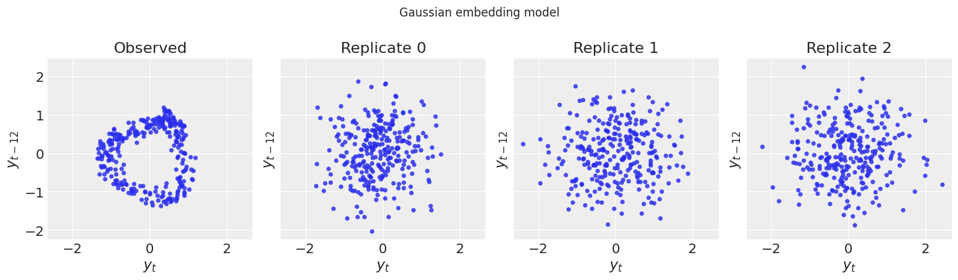
A misspecified Gaussian model on the delay embedding. It can match means and covariance but cannot reproduce the recurrent loop.
A revised Fourier seasonal model on the time series. Its posterior predictive delay embeddings recover the loop.
The example illustrates a Bayesian workflow pattern:
ordinary posterior predictive checks pass → topological posterior predictive checks detect missing recurrent structure → model is revised → topological posterior predictive checks improve.
The topology is used as an external diagnostic on posterior predictive samples. Related work has used topological summaries in likelihood-free and approximate Bayesian computation []; here the focus is posterior predictive model criticism in a standard PyMC workflow.
Dependencies#
This notebook requires PyMC, ArviZ, NumPy, Pandas, Matplotlib, and ripser for Vietoris–Rips persistent homology.
Attention
This notebook uses libraries that are not PyMC dependencies and therefore need to be installed specifically to run this notebook. Open the dropdown below for extra guidance.
Extra dependencies install instructions
In order to run this notebook (either locally or on binder) you won’t only need a working PyMC installation with all optional dependencies, but also to install some extra dependencies. For advise on installing PyMC itself, please refer to Installation
You can install these dependencies with your preferred package manager, we provide as an example the pip and conda commands below.
$ pip install
Note that if you want (or need) to install the packages from inside the notebook instead of the command line, you can install the packages by running a variation of the pip command:
import sys
!{sys.executable} -m pip install
You should not run !pip install as it might install the package in a different
environment and not be available from the Jupyter notebook even if installed.
Another alternative is using conda instead:
$ conda install
when installing scientific python packages with conda, we recommend using conda forge
The notebook intentionally keeps the example small enough to run quickly, but the Markov chain Monte Carlo cells may still take a minute or two depending on hardware.
from __future__ import annotations

import warnings

from dataclasses import dataclass
from typing import Iterable

import arviz as az
import matplotlib.pyplot as plt
import numpy as np
import pandas as pd
import pymc as pm
import pytensor.tensor as pt

try:
    from ripser import ripser
except ImportError as err:
    raise ImportError(
        "This notebook requires the `ripser` package. Install it with `pip install ripser`."
    ) from err

warnings.filterwarnings("ignore", category=FutureWarning)
warnings.filterwarnings(
    "ignore",
    message="The figure layout has changed to tight",
    category=UserWarning,
)
warnings.filterwarnings(
    "ignore",
    message="invalid value encountered in accumulate",
    category=RuntimeWarning,
)
RANDOM_SEED = 20260520
rng = np.random.default_rng(RANDOM_SEED)

az.style.use("arviz-darkgrid")
print(f"PyMC version: {pm.__version__}")
PyMC version: 5.28.5
A short intuition for homology#
Homology is a way to summarize the qualitative shape of an object. In low dimensions, the most useful summaries are intuitive:
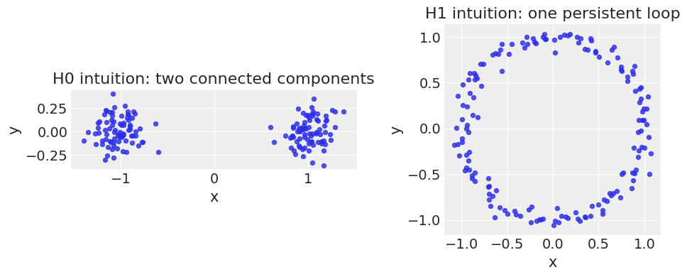
H0 tracks connected components. A point cloud with two well-separated clusters has two prominent H0 features.
H1 tracks loops or holes. A noisy circle has one prominent H1 feature.
H2 tracks enclosed voids in three-dimensional objects, such as the hollow center of a sphere.
For point-cloud data, there is no single fixed shape at the start. Persistent homology therefore builds a family of shapes indexed by a distance scale. At a small scale, each point is almost isolated. As the scale grows, nearby points connect, loops can appear, and eventually loops are filled in. A feature’s persistence is the gap between the scale where it appears and the scale where it disappears.
This is useful for posterior predictive checking because some model failures are global rather than marginal. A model can reproduce means, variances, and correlations while still failing to reproduce a connected component, a loop, or another large-scale geometric structure.
# Visual intuition: H0 sees connected components; H1 sees loops.
theta = np.linspace(0.0, 2.0 * np.pi, 160, endpoint=False)
noisy_circle = np.column_stack([np.cos(theta), np.sin(theta)])
noisy_circle += rng.normal(scale=0.06, size=noisy_circle.shape)

left_cluster = rng.normal(loc=(-1.0, 0.0), scale=0.15, size=(80, 2))
right_cluster = rng.normal(loc=(1.0, 0.0), scale=0.15, size=(80, 2))
two_clusters = np.vstack([left_cluster, right_cluster])

fig, axes = plt.subplots(1, 2, figsize=(10, 4))
axes[0].scatter(two_clusters[:, 0], two_clusters[:, 1], s=18, alpha=0.8)
axes[0].set_title("H0 intuition: two connected components")
axes[0].set_aspect("equal", adjustable="box")

axes[1].scatter(noisy_circle[:, 0], noisy_circle[:, 1], s=18, alpha=0.8)
axes[1].set_title("H1 intuition: one persistent loop")
axes[1].set_aspect("equal", adjustable="box")

for ax in axes:
    ax.set_xlabel("x")
    ax.set_ylabel("y")

plt.tight_layout()
Generate a seasonal time series#
We generate a synthetic seasonal signal with noise and a weak second harmonic. The observed data is not constructed as a literal circle. The loop appears only after delay-coordinate embedding, which is a standard way to reveal recurrence in a time series.
def make_seasonal_timeseries(
    n_time: int = 300,
    period: int = 50,
    amplitude: float = 1.0,
    noise: float = 0.15,
    trend_strength: float = 0.0,
    seed: int = RANDOM_SEED,
) -> np.ndarray:
    """Generate a noisy seasonal time series with a weak second harmonic.

    The signal is deliberately simple: it is periodic, mildly non-sinusoidal,
    and noisy. This makes it useful for demonstrating how a delay embedding can
    reveal recurrent structure that is not explicit in the one-dimensional time
    series plot.
    """
    rng = np.random.default_rng(seed)
    t = np.arange(n_time, dtype=float)
    seasonal = amplitude * np.sin(2.0 * np.pi * t / period)
    harmonic = 0.25 * amplitude * np.sin(4.0 * np.pi * t / period + 0.7)
    trend = trend_strength * (t - t.mean()) / max(t.max(), 1.0)
    y = seasonal + harmonic + trend + rng.normal(scale=noise, size=n_time)
    return y.astype(float)


def delay_embedding(y: np.ndarray, lag: int = 12, dim: int = 2) -> np.ndarray:
    """Return a delay-coordinate embedding of a univariate time series.

    The output has columns ``(y_t, y_{t-lag}, ...)``. For periodic or recurrent
    signals, this embedding can turn temporal recurrence into visible geometric
    structure, such as a loop. That geometry is what the topological posterior
    predictive check compares between observed and replicated data.
    """
    y = np.asarray(y, dtype=float)
    if lag <= 0:
        raise ValueError("lag must be positive")
    if dim < 2:
        raise ValueError("dim must be at least 2")
    n_points = len(y) - (dim - 1) * lag
    if n_points <= 5:
        raise ValueError("time series is too short for the requested delay embedding")
    cols = [y[(dim - 1 - j) * lag : (dim - 1 - j) * lag + n_points] for j in range(dim)]
    return np.column_stack(cols)


N_TIME = 300
PERIOD = 50
LAG = 12
DELAY_DIM = 2

# The lag is approximately one quarter of the period, which makes the recurrent loop visible.
observed_series = make_seasonal_timeseries(
    n_time=N_TIME, period=PERIOD, noise=0.15, seed=RANDOM_SEED
)
observed_embedding = delay_embedding(observed_series, lag=LAG, dim=DELAY_DIM)

fig, axes = plt.subplots(1, 2, figsize=(11, 4))
axes[0].plot(observed_series, lw=1.5)
axes[0].set(title="Observed seasonal time series", xlabel="time", ylabel="y")
axes[1].scatter(observed_embedding[:, 0], observed_embedding[:, 1], s=16, alpha=0.8)
axes[1].set(title="Delay-coordinate embedding", xlabel="$y_t$", ylabel=f"$y_{{t-{LAG}}}$")
axes[1].set_aspect("equal", adjustable="box")
plt.tight_layout()
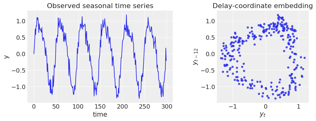
The delay embedding has an annular or loop-like shape. A model that treats the embedded points as a single Gaussian cloud can match the embedding’s mean and covariance, but it has no reason to preserve the hole.
Topological posterior predictive check helper functions#
For each posterior predictive replicate, we compute Vietoris–Rips persistent homology with ripser. We summarize the diagrams using a few scalar summaries:
h1_max_persistence: the longest-lived loop;h1_persistence_gap: the gap between the longest and second-longest loop lifetimes;h1_total_persistence_p2: squared total H1 persistence, which emphasizes large features;h1_n_features_ge_threshold: number of loops with lifetime above a threshold.
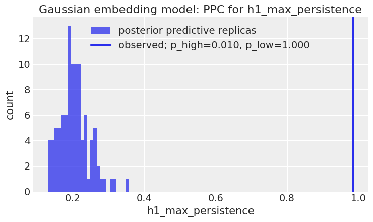
For this example, the main diagnostic is h1_max_persistence.
Diagram = np.ndarray
Diagrams = list[Diagram]


@dataclass
class TopoPPCResult:
    """Container for ordinary and topological posterior predictive check results."""

    name: str
    observed_embedding: np.ndarray
    replicated_embeddings: np.ndarray
    obs_diagrams: Diagrams
    rep_diagrams: list[Diagrams]
    ordinary_table: pd.DataFrame
    topo_table: pd.DataFrame


def compute_persistence_diagrams(X: np.ndarray, maxdim: int = 1) -> Diagrams:
    """Compute Vietoris--Rips persistence diagrams for a point cloud.

    ``ripser`` returns one diagram per homological dimension. In this notebook,
    dimension 0 tracks connected components and dimension 1 tracks loops.
    """
    return ripser(X, maxdim=maxdim)["dgms"]


def finite_lifetimes(diagram: Diagram) -> np.ndarray:
    """Return finite persistence lifetimes from a persistence diagram."""
    if diagram is None or diagram.size == 0:
        return np.array([], dtype=float)
    dgm = np.asarray(diagram, dtype=float)
    dgm = dgm[np.isfinite(dgm[:, 1])]
    if dgm.size == 0:
        return np.array([], dtype=float)
    return np.maximum(dgm[:, 1] - dgm[:, 0], 0.0)


def max_persistence(diagram: Diagram) -> float:
    """Return the lifetime of the longest-lived topological feature."""
    lifetimes = finite_lifetimes(diagram)
    return float(np.max(lifetimes)) if lifetimes.size else 0.0


def second_max_persistence(diagram: Diagram) -> float:
    """Return the second-largest finite lifetime, or zero if it is absent."""
    lifetimes = finite_lifetimes(diagram)
    if lifetimes.size < 2:
        return 0.0
    return float(np.sort(lifetimes)[-2])


def persistence_gap(diagram: Diagram) -> float:
    """Return the gap between the two longest-lived topological features."""
    return float(max_persistence(diagram) - second_max_persistence(diagram))


def total_persistence(diagram: Diagram, power: float = 1.0) -> float:
    """Return total persistence, optionally emphasizing long-lived features."""
    lifetimes = finite_lifetimes(diagram)
    return float(np.sum(lifetimes**power)) if lifetimes.size else 0.0


def n_persistent_features(diagram: Diagram, threshold: float) -> int:
    """Count features whose lifetimes exceed a chosen persistence threshold."""
    lifetimes = finite_lifetimes(diagram)
    return int(np.sum(lifetimes >= threshold))


def summarize_diagram(diagram: Diagram, dim: int, threshold: float = 0.5) -> dict[str, float]:
    """Convert one persistence diagram into scalar discrepancy statistics."""
    prefix = f"h{dim}"
    return {
        f"{prefix}_n_finite_features": float(finite_lifetimes(diagram).size),
        f"{prefix}_max_persistence": max_persistence(diagram),
        f"{prefix}_second_max_persistence": second_max_persistence(diagram),
        f"{prefix}_persistence_gap": persistence_gap(diagram),
        f"{prefix}_total_persistence_p1": total_persistence(diagram, power=1.0),
        f"{prefix}_total_persistence_p2": total_persistence(diagram, power=2.0),
        f"{prefix}_n_features_ge_threshold": float(n_persistent_features(diagram, threshold)),
    }


def smoothed_ppc_p_value(
    obs_value: float, rep_values: Iterable[float], direction: str = "greater"
) -> float:
    """Compute a conservative Monte Carlo posterior predictive p-value.

    The +1 smoothing avoids returning exactly zero when the observed statistic
    is more extreme than all finite posterior predictive draws.
    """
    values = np.asarray(list(rep_values), dtype=float)
    p_greater = (1.0 + np.sum(values >= obs_value)) / (values.size + 1.0)
    p_less = (1.0 + np.sum(values <= obs_value)) / (values.size + 1.0)
    if direction == "greater":
        return float(p_greater)
    if direction == "less":
        return float(p_less)
    if direction == "two-sided":
        return float(min(1.0, 2.0 * min(p_greater, p_less)))
    raise ValueError(f"unknown direction: {direction}")


def ordinary_embedding_table(
    observed_embedding: np.ndarray, replicated_embeddings: np.ndarray
) -> pd.DataFrame:
    """Compare mean and covariance summaries of observed and replicated embeddings."""

    def summarize(X: np.ndarray) -> dict[str, float]:
        mean = X.mean(axis=0)
        cov = np.cov(X.T)
        eigvals = np.linalg.eigvalsh(cov)
        return {
            "mean_x": float(mean[0]),
            "mean_y": float(mean[1]),
            "cov_xx": float(cov[0, 0]),
            "cov_yy": float(cov[1, 1]),
            "cov_xy": float(cov[0, 1]),
            "cov_eig_min": float(eigvals[0]),
            "cov_eig_max": float(eigvals[-1]),
        }

    obs_summary = summarize(observed_embedding)
    rep_summaries = pd.DataFrame([summarize(X) for X in replicated_embeddings])
    rows = []
    for metric, observed in obs_summary.items():
        rep_values = rep_summaries[metric].to_numpy()
        q05, q50, q95 = np.quantile(rep_values, [0.05, 0.50, 0.95])
        rows.append(
            {
                "metric": metric,
                "observed": observed,
                "rep_q05": q05,
                "rep_q50": q50,
                "rep_q95": q95,
                "inside_90_interval": bool(q05 <= observed <= q95),
            }
        )
    return pd.DataFrame(rows)


def topological_table(
    obs_diagrams: Diagrams, rep_diagrams: list[Diagrams], h1_threshold: float = 0.5
) -> pd.DataFrame:
    """Compare observed topological summaries to posterior predictive summaries."""
    obs_summary = {}
    for dim in [0, 1]:
        obs_summary.update(summarize_diagram(obs_diagrams[dim], dim=dim, threshold=h1_threshold))

    rep_rows = []
    for diagrams in rep_diagrams:
        row = {}
        for dim in [0, 1]:
            row.update(summarize_diagram(diagrams[dim], dim=dim, threshold=h1_threshold))
        rep_rows.append(row)
    rep_summary = pd.DataFrame(rep_rows)

    rows = []
    for metric, observed in obs_summary.items():
        rep_values = rep_summary[metric].to_numpy(dtype=float)
        q05, q50, q95 = np.quantile(rep_values, [0.05, 0.50, 0.95])
        rows.append(
            {
                "metric": metric,
                "observed": observed,
                "rep_q05": q05,
                "rep_q50": q50,
                "rep_q95": q95,
                "p_high": smoothed_ppc_p_value(observed, rep_values, "greater"),
                "p_low": smoothed_ppc_p_value(observed, rep_values, "less"),
                "p_two_sided": smoothed_ppc_p_value(observed, rep_values, "two-sided"),
            }
        )
    return pd.DataFrame(rows)


def run_topoppc(
    name: str,
    observed_embedding: np.ndarray,
    replicated_embeddings: np.ndarray,
    h1_threshold: float = 0.5,
) -> TopoPPCResult:
    """Run ordinary and topological posterior predictive checks for embeddings."""
    obs_diagrams = compute_persistence_diagrams(observed_embedding, maxdim=1)
    rep_diagrams = [compute_persistence_diagrams(X, maxdim=1) for X in replicated_embeddings]
    return TopoPPCResult(
        name=name,
        observed_embedding=observed_embedding,
        replicated_embeddings=replicated_embeddings,
        obs_diagrams=obs_diagrams,
        rep_diagrams=rep_diagrams,
        ordinary_table=ordinary_embedding_table(observed_embedding, replicated_embeddings),
        topo_table=topological_table(obs_diagrams, rep_diagrams, h1_threshold=h1_threshold),
    )
def plot_replicates(result: TopoPPCResult, rep_ids: tuple[int, ...] = (0, 1, 2)) -> None:
    """Plot the observed embedding next to a few posterior predictive embeddings."""
    fig, axes = plt.subplots(1, 1 + len(rep_ids), figsize=(14, 3.6), sharex=True, sharey=True)
    axes[0].scatter(
        result.observed_embedding[:, 0], result.observed_embedding[:, 1], s=13, alpha=0.8
    )
    axes[0].set_title("Observed")
    axes[0].set_aspect("equal", adjustable="box")
    for ax, rep_id in zip(axes[1:], rep_ids):
        X = result.replicated_embeddings[rep_id]
        ax.scatter(X[:, 0], X[:, 1], s=13, alpha=0.8)
        ax.set_title(f"Replicate {rep_id}")
        ax.set_aspect("equal", adjustable="box")
    for ax in axes:
        ax.set_xlabel("$y_t$")
        ax.set_ylabel(f"$y_{{t-{LAG}}}$")
    fig.suptitle(result.name, y=1.05)
    plt.tight_layout()


def plot_metric_histogram(result: TopoPPCResult, metric: str) -> None:
    """Plot the posterior predictive distribution of one topological statistic."""
    row = result.topo_table.query("metric == @metric").iloc[0]
    obs = float(row["observed"])

    # Recompute replicated scalar values from diagrams for plotting.
    dim = int(metric[1])
    values = []
    for diagrams in result.rep_diagrams:
        summary = summarize_diagram(diagrams[dim], dim=dim)
        values.append(summary[metric])
    values = np.asarray(values)

    fig, ax = plt.subplots(figsize=(7.5, 4.5))
    ax.hist(values, bins=25, alpha=0.75, label="posterior predictive replicas")
    ax.axvline(
        obs,
        lw=2.5,
        label=f"observed; p_high={row['p_high']:.3f}, p_low={row['p_low']:.3f}",
    )
    ax.set(title=f"{result.name}: PPC for {metric}", xlabel=metric, ylabel="count")
    ax.legend()
    plt.tight_layout()


def plot_h1_diagram(result: TopoPPCResult, rep_id: int = 0) -> None:
    """Plot finite H1 birth/death pairs for the observed data and one replicate."""
    obs = result.obs_diagrams[1]
    rep = result.rep_diagrams[rep_id][1]
    obs = obs[np.isfinite(obs[:, 1])] if obs.size else np.empty((0, 2))
    rep = rep[np.isfinite(rep[:, 1])] if rep.size else np.empty((0, 2))

    fig, ax = plt.subplots(figsize=(5.5, 5))
    if rep.size:
        ax.scatter(rep[:, 0], rep[:, 1], s=25, alpha=0.55, label=f"replicate {rep_id}")
    if obs.size:
        ax.scatter(obs[:, 0], obs[:, 1], s=35, alpha=0.85, label="observed")
    if obs.size or rep.size:
        stacked = np.vstack([x for x in [obs, rep] if x.size])
        hi = float(np.max(stacked[:, 1])) * 1.05
    else:
        hi = 1.0
    ax.plot([0, hi], [0, hi], ls="--", lw=1.5, label="death = birth")
    ax.set(xlabel="birth", ylabel="death", title=f"{result.name}: finite H1 persistence diagram")
    ax.set_xlim(0, hi)
    ax.set_ylim(0, hi)
    ax.legend()
    plt.tight_layout()


def display_selected_tables(result: TopoPPCResult) -> None:
    """Display compact ordinary and topological posterior predictive check tables."""
    selected_metrics = [
        "h1_max_persistence",
        "h1_persistence_gap",
        "h1_total_persistence_p2",
        "h1_n_features_ge_threshold",
        "h0_max_persistence",
    ]
    print("Ordinary PPC table")
    display(result.ordinary_table)
    print("Selected topological PPC table")
    display(result.topo_table[result.topo_table["metric"].isin(selected_metrics)])


def replace_inf_deaths(diagram: Diagram, max_eps: float) -> Diagram:
    """Replace infinite deaths by ``max_eps`` for bounded Betti-curve plotting."""
    if diagram is None or diagram.size == 0:
        return np.empty((0, 2), dtype=float)
    dgm = np.asarray(diagram, dtype=float).copy()
    dgm[np.isinf(dgm[:, 1]), 1] = max_eps
    return dgm


def betti_curve(diagram: Diagram, eps_grid: np.ndarray, max_eps: float) -> np.ndarray:
    """Compute a Betti curve from a persistence diagram over a grid of scales."""
    dgm = replace_inf_deaths(diagram, max_eps=max_eps)
    if dgm.size == 0:
        return np.zeros_like(eps_grid, dtype=float)

    births = dgm[:, 0]
    deaths = dgm[:, 1]
    curve = np.zeros_like(eps_grid, dtype=float)
    for i, eps in enumerate(eps_grid):
        curve[i] = np.sum((births <= eps) & (eps < deaths))
    return curve


def betti_curves_for_result(
    result: TopoPPCResult,
    dim: int = 1,
    n_grid: int = 200,
    eps_max_quantile: float = 0.95,
) -> tuple[np.ndarray, np.ndarray, np.ndarray]:
    """Return observed and replicated Betti curves for one homological dimension."""
    finite_deaths = []
    for dgm in [result.obs_diagrams[dim]] + [dgms[dim] for dgms in result.rep_diagrams]:
        if dgm.size:
            finite_deaths.extend(dgm[np.isfinite(dgm[:, 1]), 1].tolist())

    max_eps = float(np.quantile(finite_deaths, eps_max_quantile)) if finite_deaths else 1.0
    max_eps = max(max_eps, 1e-8)
    eps_grid = np.linspace(0.0, max_eps, n_grid)

    obs_curve = betti_curve(result.obs_diagrams[dim], eps_grid, max_eps=max_eps)
    rep_curves = np.vstack(
        [betti_curve(dgms[dim], eps_grid, max_eps=max_eps) for dgms in result.rep_diagrams]
    )
    return eps_grid, obs_curve, rep_curves


def plot_betti_envelope(result: TopoPPCResult, dim: int = 1) -> None:
    """Plot an observed Betti curve against its posterior predictive envelope."""
    eps_grid, obs_curve, rep_curves = betti_curves_for_result(result, dim=dim)

    q05 = np.quantile(rep_curves, 0.05, axis=0)
    q25 = np.quantile(rep_curves, 0.25, axis=0)
    q50 = np.quantile(rep_curves, 0.50, axis=0)
    q75 = np.quantile(rep_curves, 0.75, axis=0)
    q95 = np.quantile(rep_curves, 0.95, axis=0)

    fig, ax = plt.subplots(figsize=(8, 4.8))
    ax.fill_between(eps_grid, q05, q95, alpha=0.20, label="posterior predictive 90% envelope")
    ax.fill_between(eps_grid, q25, q75, alpha=0.35, label="posterior predictive 50% envelope")
    ax.plot(eps_grid, q50, ls="--", label="posterior predictive median")
    ax.plot(eps_grid, obs_curve, lw=2.5, label="observed")
    ax.set(
        xlabel="filtration scale epsilon",
        ylabel=f"Betti-{dim}",
        title=f"{result.name}: Betti-{dim} posterior predictive envelope",
    )
    ax.legend()
    plt.tight_layout()
Model 1: a Gaussian model on the delay embedding#
The first model treats the delay-embedded points as independent draws from a single bivariate normal distribution. This is deliberately misspecified: a Gaussian cloud can reproduce mean and covariance, but it cannot express the recurrent hole in the embedding.
coords_bad = {
    "obs_id": np.arange(observed_embedding.shape[0]),
    "coord": ["y_t", f"y_t_minus_{LAG}"],
}

with pm.Model(coords=coords_bad) as gaussian_embedding_model:
    mu = pm.Normal("mu", mu=0.0, sigma=2.0, dims="coord")
    chol, corr, stds = pm.LKJCholeskyCov(
        "chol_cov",
        n=2,
        eta=2.0,
        sd_dist=pm.Exponential.dist(1.0),
        compute_corr=True,
    )
    x = pm.MvNormal("x", mu=mu, chol=chol, observed=observed_embedding, dims=("obs_id", "coord"))

    idata_bad = pm.sample(
        draws=400,
        tune=400,
        chains=2,
        cores=1,
        target_accept=0.9,
        random_seed=RANDOM_SEED,
        progressbar=False,
    )
    ppc_bad = pm.sample_posterior_predictive(
        idata_bad,
        var_names=["x"],
        random_seed=RANDOM_SEED + 1,
        progressbar=False,
    )
az.summary(idata_bad, var_names=["mu", "chol_cov_stds"], round_to=2)

rhat_bad = az.rhat(idata_bad, var_names=["mu", "chol_cov_stds"]).to_array()
assert float(rhat_bad.max()) < 1.03
def posterior_predictive_embedding_array(
    ppc,
    var_name: str = "x",
    n_rep: int = 100,
    seed: int = RANDOM_SEED,
) -> np.ndarray:
    """Extract a manageable subset of posterior predictive embedding replicas."""
    arr = ppc.posterior_predictive[var_name]
    arr = arr.stack(sample=("chain", "draw")).transpose("sample", "obs_id", "coord").values
    rng = np.random.default_rng(seed)
    idx = rng.choice(arr.shape[0], size=min(n_rep, arr.shape[0]), replace=False)
    return arr[idx]


replicated_embeddings_bad = posterior_predictive_embedding_array(ppc_bad, var_name="x", n_rep=100)
bad_result = run_topoppc(
    "Gaussian embedding model", observed_embedding, replicated_embeddings_bad, h1_threshold=0.5
)

display_selected_tables(bad_result)
plot_replicates(bad_result)
plot_metric_histogram(bad_result, "h1_max_persistence")
plot_h1_diagram(bad_result, rep_id=0)
plot_betti_envelope(bad_result, dim=1)
Ordinary PPC table
| metric | observed | rep_q05 | rep_q50 | rep_q95 | inside_90_interval | |
|---|---|---|---|---|---|---|
| 0 | mean_x | -0.029305 | -0.121837 | -0.042997 | 0.066254 | True |
| 1 | mean_y | 0.032757 | -0.058779 | 0.037590 | 0.129806 | True |
| 2 | cov_xx | 0.532998 | 0.461431 | 0.545668 | 0.659702 | True |
| 3 | cov_yy | 0.525348 | 0.449583 | 0.523734 | 0.632085 | True |
| 4 | cov_xy | 0.023766 | -0.052610 | 0.021923 | 0.099306 | True |
| 5 | cov_eig_min | 0.505101 | 0.402274 | 0.476335 | 0.565186 | True |
| 6 | cov_eig_max | 0.553244 | 0.517281 | 0.596644 | 0.702918 | True |
Selected topological PPC table
| metric | observed | rep_q05 | rep_q50 | rep_q95 | p_high | p_low | p_two_sided | |
|---|---|---|---|---|---|---|---|---|
| 1 | h0_max_persistence | 0.214557 | 0.523941 | 0.756681 | 1.102609 | 1.000000 | 0.009901 | 0.019802 |
| 8 | h1_max_persistence | 0.983425 | 0.145451 | 0.201963 | 0.273901 | 0.009901 | 1.000000 | 0.019802 |
| 10 | h1_persistence_gap | 0.882811 | 0.001986 | 0.022538 | 0.101508 | 0.009901 | 1.000000 | 0.019802 |
| 12 | h1_total_persistence_p2 | 1.021367 | 0.203647 | 0.283310 | 0.386262 | 0.009901 | 1.000000 | 0.019802 |
| 13 | h1_n_features_ge_threshold | 1.000000 | 0.000000 | 0.000000 | 0.000000 | 0.009901 | 1.000000 | 0.019802 |
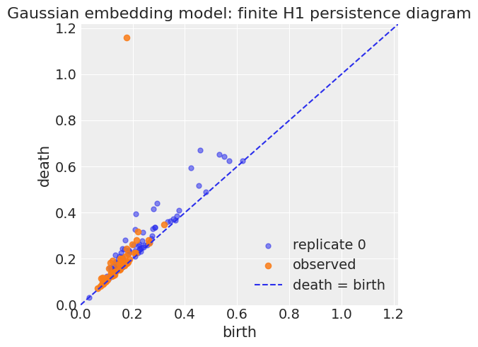
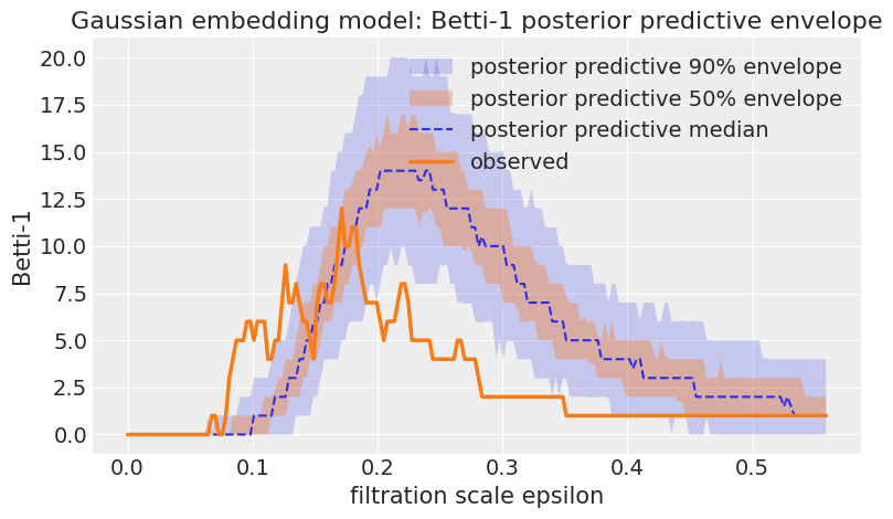
The scalar diagnostic below is the primary decision statistic, but the Betti-1 envelope is also useful as a visual posterior predictive check. It shows how the number of active one-dimensional holes evolves over the filtration scale, while the maximum-persistence statistic focuses on the single most persistent loop.
The Gaussian model usually passes the ordinary mean/covariance checks. But the topological check based on h1_max_persistence should fail: the observed delay embedding contains one persistent loop, while the Gaussian posterior predictive replicas contain only short-lived noisy cycles.
Model 2: a revised Fourier seasonal model#
The topological failure suggests that the model is missing recurrence or periodic structure. We therefore fit a simple Fourier seasonal regression to the original time series, generate posterior predictive time series, and then delay-embed those posterior predictive samples.
This is the key workflow step: the topology is not forced into the sampler. Instead, the topological posterior predictive check diagnoses a structural failure and motivates a better generative model.
def fourier_design(t: np.ndarray, period: int, harmonics: int = 2) -> np.ndarray:
    """Build an intercept plus sine/cosine Fourier design matrix."""
    t = np.asarray(t, dtype=float)
    cols = [np.ones_like(t)]
    for h in range(1, harmonics + 1):
        cols.append(np.sin(2.0 * np.pi * h * t / period))
        cols.append(np.cos(2.0 * np.pi * h * t / period))
    return np.column_stack(cols)


HARMONICS = 2
time = np.arange(N_TIME)
fourier_design_matrix = fourier_design(time, period=PERIOD, harmonics=HARMONICS)

coords_good = {
    "time": time,
    "coef": ["intercept"]
    + [f"h{h}_{kind}" for h in range(1, HARMONICS + 1) for kind in ["sin", "cos"]],
}

with pm.Model(coords=coords_good) as fourier_model:
    beta = pm.Normal("beta", mu=0.0, sigma=1.5, dims="coef")
    sigma = pm.HalfNormal("sigma", sigma=0.5)
    mu = pt.dot(fourier_design_matrix, beta)
    y = pm.Normal("y", mu=mu, sigma=sigma, observed=observed_series, dims="time")

    idata_good = pm.sample(
        draws=400,
        tune=400,
        chains=2,
        cores=1,
        target_accept=0.9,
        random_seed=RANDOM_SEED + 2,
        progressbar=False,
    )
    ppc_good = pm.sample_posterior_predictive(
        idata_good,
        var_names=["y"],
        random_seed=RANDOM_SEED + 3,
        progressbar=False,
    )
az.summary(idata_good, var_names=["beta", "sigma"], round_to=2)

rhat_good = az.rhat(idata_good, var_names=["beta", "sigma"]).to_array()
assert float(rhat_good.max()) < 1.03
def posterior_predictive_delay_embeddings(
    ppc,
    var_name: str = "y",
    lag: int = LAG,
    dim: int = DELAY_DIM,
    n_rep: int = 100,
    seed: int = RANDOM_SEED,
) -> np.ndarray:
    """Delay-embed posterior predictive time series replicas."""
    arr = ppc.posterior_predictive[var_name]
    arr = arr.stack(sample=("chain", "draw")).transpose("sample", "time").values
    rng = np.random.default_rng(seed)
    idx = rng.choice(arr.shape[0], size=min(n_rep, arr.shape[0]), replace=False)
    return np.stack([delay_embedding(arr[i], lag=lag, dim=dim) for i in idx], axis=0)


replicated_embeddings_good = posterior_predictive_delay_embeddings(
    ppc_good, var_name="y", n_rep=100
)
good_result = run_topoppc(
    "Fourier seasonal model", observed_embedding, replicated_embeddings_good, h1_threshold=0.5
)

display_selected_tables(good_result)
plot_replicates(good_result)
plot_metric_histogram(good_result, "h1_max_persistence")
plot_h1_diagram(good_result, rep_id=0)
plot_betti_envelope(good_result, dim=1)
Ordinary PPC table
| metric | observed | rep_q05 | rep_q50 | rep_q95 | inside_90_interval | |
|---|---|---|---|---|---|---|
| 0 | mean_x | -0.029305 | -0.047377 | -0.027848 | -0.009451 | True |
| 1 | mean_y | 0.032757 | 0.014827 | 0.034417 | 0.053334 | True |
| 2 | cov_xx | 0.532998 | 0.506676 | 0.535881 | 0.565044 | True |
| 3 | cov_yy | 0.525348 | 0.499539 | 0.527085 | 0.559601 | True |
| 4 | cov_xy | 0.023766 | 0.014404 | 0.023014 | 0.028887 | True |
| 5 | cov_eig_min | 0.505101 | 0.479236 | 0.509354 | 0.542066 | True |
| 6 | cov_eig_max | 0.553244 | 0.526374 | 0.552686 | 0.585372 | True |
Selected topological PPC table
| metric | observed | rep_q05 | rep_q50 | rep_q95 | p_high | p_low | p_two_sided | |
|---|---|---|---|---|---|---|---|---|
| 1 | h0_max_persistence | 0.214557 | 0.207123 | 0.256732 | 0.368526 | 0.910891 | 0.099010 | 0.198020 |
| 8 | h1_max_persistence | 0.983425 | 0.717392 | 0.919905 | 1.011457 | 0.128713 | 0.881188 | 0.257426 |
| 10 | h1_persistence_gap | 0.882811 | 0.625601 | 0.821610 | 0.927079 | 0.188119 | 0.821782 | 0.376238 |
| 12 | h1_total_persistence_p2 | 1.021367 | 0.566306 | 0.901111 | 1.078509 | 0.138614 | 0.871287 | 0.277228 |
| 13 | h1_n_features_ge_threshold | 1.000000 | 1.000000 | 1.000000 | 1.000000 | 1.000000 | 1.000000 | 1.000000 |
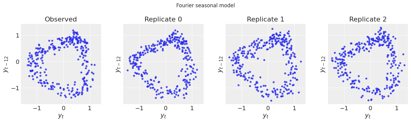
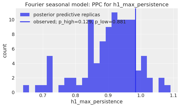
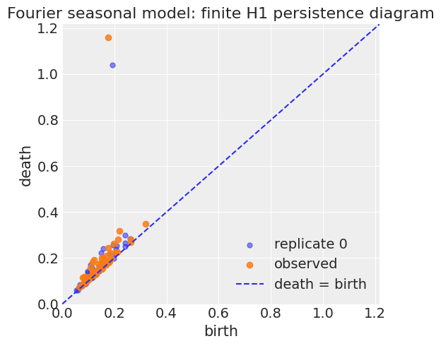
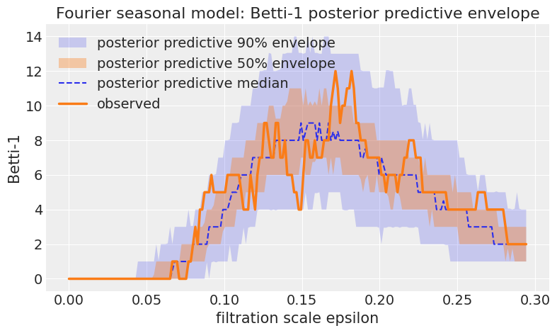
After adding seasonal structure, the posterior predictive delay embeddings should now reproduce the observed loop. The h1_max_persistence value for the observed data should be typical under the revised model’s posterior predictive distribution.
Compare the two models through the topological posterior predictive check#
The table below compares the main topological discrepancy, h1_max_persistence, between the misspecified Gaussian embedding model and the revised Fourier seasonal model.
def extract_metric(result: TopoPPCResult, metric: str) -> pd.Series:
    """Extract one discrepancy row and attach the model name."""
    row = result.topo_table.query("metric == @metric").iloc[0].copy()
    row["model"] = result.name
    return row


comparison = pd.DataFrame(
    [
        extract_metric(bad_result, "h1_max_persistence"),
        extract_metric(good_result, "h1_max_persistence"),
    ]
)[["model", "observed", "rep_q05", "rep_q50", "rep_q95", "p_high", "p_low", "p_two_sided"]]
comparison
| model | observed | rep_q05 | rep_q50 | rep_q95 | p_high | p_low | p_two_sided | |
|---|---|---|---|---|---|---|---|---|
| 8 | Gaussian embedding model | 0.983425 | 0.145451 | 0.201963 | 0.273901 | 0.009901 | 1.000000 | 0.019802 |
| 8 | Fourier seasonal model | 0.983425 | 0.717392 | 0.919905 | 1.011457 | 0.128713 | 0.881188 | 0.257426 |
The intended interpretation is:
The Gaussian embedding model can pass ordinary moment-based posterior predictive checks but fails the topological posterior predictive check because it cannot reproduce the recurrent loop.
The Fourier seasonal model is structurally closer to the data-generating process and produces posterior predictive delay embeddings with similar H1 persistence to the observed embedding.
This demonstrates how persistent homology can be used as a model criticism tool: it detects a missing global shape feature and suggests a direction for model revision.
Discussion and limitations#
Topological posterior predictive checks should not replace ordinary posterior predictive checks. They answer a different question: whether the posterior predictive distribution reproduces the global shape of the observed data in a chosen representation. In this notebook, the representation is a delay-coordinate embedding of a time series.
Several choices matter:
the data representation used before computing topology;
the filtration and persistent homology dimension;
the scalar topological summary used as a discrepancy;
the number of posterior predictive replicates;
whether the topological feature is scientifically meaningful rather than an artifact of preprocessing.
The method is most useful when the scientific question involves recurrence, loops, disconnected components, branching structure, voids, or other global geometric features.
A conservative way to phrase the contribution is:
Persistent homology summaries can be used as posterior predictive discrepancy statistics in Bayesian workflow, allowing model criticism for global shape features that ordinary scalar summaries may miss.
Appendix: why homology works for point clouds#
This section gives a compact mathematical view of the construction used above. It is not needed to use the diagnostic, but it explains why persistent homology is a natural source of discrepancy statistics.
A simplicial complex is a shape built from vertices, edges, triangles, tetrahedra, and their higher-dimensional analogues. For a point cloud, the Vietoris–Rips construction builds such a complex at a distance scale \(\epsilon\): points become vertices, nearby pairs become edges, triples whose pairwise distances are small become filled triangles, and so on.
For each dimension \(k\), a \(k\)-chain is a formal sum of \(k\)-simplices. The boundary operator \(\partial_k\) maps each \(k\)-simplex to its oriented boundary. For example, the boundary of an edge is its two endpoints, and the boundary of a triangle is its three edges. A central identity is
which says that the boundary of a boundary is empty.
Homology compares two kinds of objects:
cycles, which have zero boundary and therefore look closed;
boundaries, which are cycles that bound a higher-dimensional filled object.
The \(k\)-th homology group is
Its rank is the Betti number \(\beta_k\). In the examples above, \(\beta_0\) counts connected components and \(\beta_1\) counts loops that have not yet been filled by triangles.
Persistent homology repeats this calculation over a sequence of scales. A loop may be born when enough edges connect around a hole, and it may die when enough triangles fill the hole. Long persistence means that the feature is stable across scales, which is why maximum H1 persistence is a useful statistic for detecting the recurrent loop in the delay embedding.
In practice, this notebook delegates the matrix-reduction algorithm to ripser. The Bayesian workflow only needs the resulting diagrams and their scalar summaries, which can be compared to posterior predictive replicas like any other discrepancy statistic.
References#
Andrew Gelman, John B. Carlin, Hal S. Stern, David B. Dunson, Aki Vehtari, and Donald B. Rubin. Bayesian Data Analysis. Chapman and Hall/CRC, 2013.
Herbert Edelsbrunner and John Harer. Computational Topology: An Introduction. American Mathematical Society, 2010. ISBN 978-0-8218-4925-5.
Robert Ghrist. Barcodes: the persistent topology of data. Bulletin of the American Mathematical Society, 45(1):61–75, 2008. doi:10.1090/S0273-0979-07-01191-3.
Watermark#
%load_ext watermark
%watermark -n -u -v -iv -w -p pytensor,xarray
Last updated: Sun, 21 Jun 2026

Python implementation: CPython
Python version       : 3.12.13
IPython version      : 7.34.0

pytensor: 2.38.3
xarray  : 2025.12.0

arviz     : 0.22.0
matplotlib: 3.10.0
numpy     : 2.0.2
pandas    : 2.2.2
pymc      : 5.28.5
pytensor  : 2.38.3
ripser    : 0.6.15

Watermark: 2.6.0
License notice#
All the notebooks in this example gallery are provided under the MIT License which allows modification, and redistribution for any use provided the copyright and license notices are preserved.
Citing PyMC examples#
To cite this notebook, use the DOI provided by Zenodo for the pymc-examples repository.
Important
Many notebooks are adapted from other sources: blogs, books… In such cases you should cite the original source as well.
Also remember to cite the relevant libraries used by your code.
Here is an citation template in bibtex:
@incollection{citekey,
  author    = "<notebook authors, see above>",
  title     = "<notebook title>",
  editor    = "PyMC Team",
  booktitle = "PyMC examples",
  doi       = "10.5281/zenodo.5654871"
}
which once rendered could look like: